
Mobile Robot Autonomous Navigation: SLAM & A*
This project included building, calibrating, and programming a differential‑drive MBot (Jetson Nano, magnetic wheel encoders, 2D LiDAR, and 3‑axis MEMS IMU) to go from raw hardware to map‑aware autonomy. The stack covers feed‑forward + PID wheel control, gyrodometry, occupancy‑grid mapping, Monte Carlo Localization (MCL), SLAM integration, A* path planning, and frontier exploration.
System Overview
The pipeline breaks into Action (Control), Perception (Mapping & Sensing), and Reasoning (Planning & Exploration):
- Action: PWM feed‑forward from wheel speed calibration + PID feedback. A high‑level RTR (Rotate–Translate–Rotate) motion controller executes waypoint motion.
- Perception: LiDAR occupancy grid via Bresenham raytracing; IMU‑aided odometry (gyrodometry); AprilTag‑assisted routines for vision navigation experiments.
- Reasoning: Particle‑filter MCL on the grid; A* search on an 8‑connected lattice; frontier detection (free‑adjacent‑to‑unknown) for autonomous exploration.
Platform & Hardware
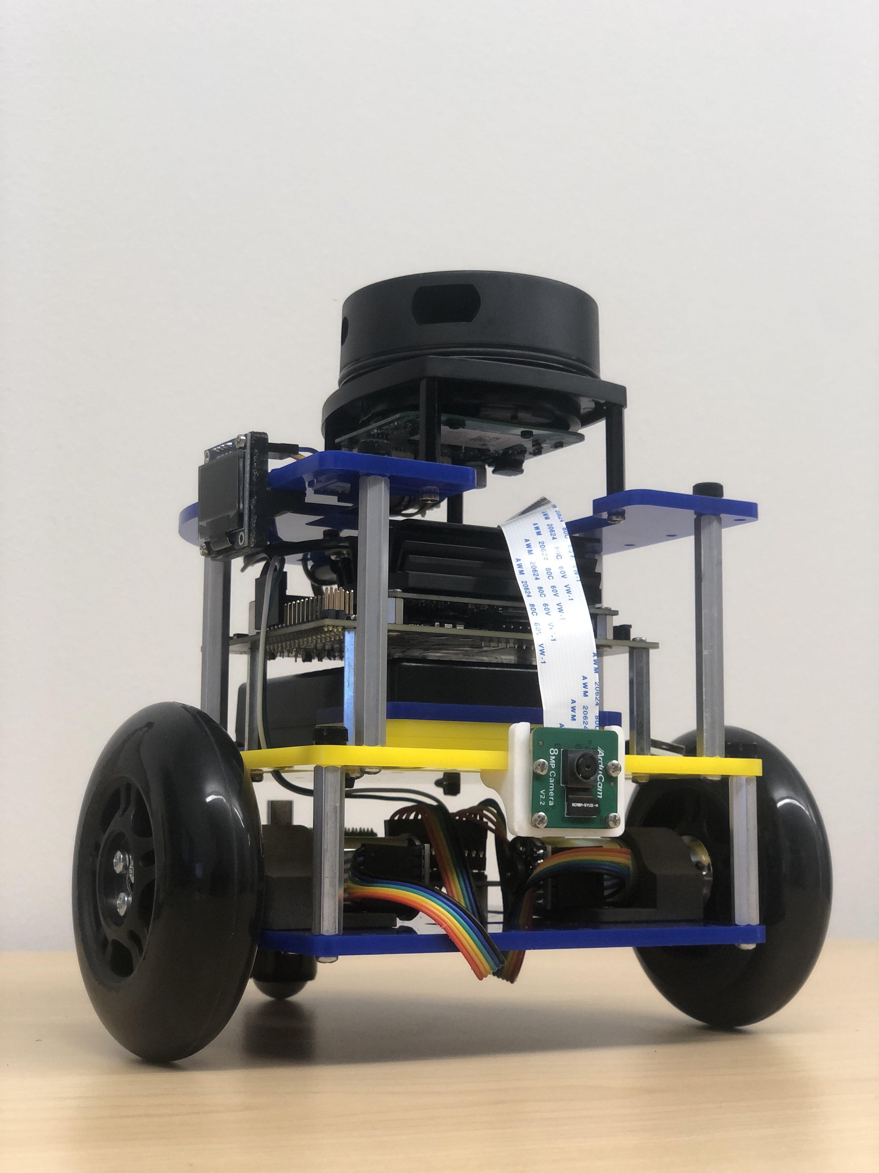
- MBot (Classic) differential‑drive base
- Jetson Nano + driver board
- Magnetic encoders (per wheel)
- 2D LiDAR, 3‑axis MEMS IMU
Control Stack
Calibration, state estimation, and motion control share one loop so the robot can follow commanded paths while rejecting drift and bias.
- Calibration: Determine motor and encoder polarities plus the commanded‑speed → PWM map (
PWM = m·v + b). Multiple trials per wheel/direction provide feed‑forward terms and priors for tuning. - Gyrodometry: Fuse encoders with the IMU gyro so heading stays stable through slip; sanity checks show 1.0 m/s commands yield ≈ 0.53 m forward with minor lateral drift, and 3.14 rad/s spins reach ≈ 150°/s.
- PID Velocity Control: Tighten wheel tracking around the feed‑forward setpoint with
Kp = 0.001,Kd = 0.001,Ki = 0.002, plus low‑pass filtering and accel limits to prevent slip. - RTR Motion Layer: Execute waypoints via Rotate→Translate→Rotate segments, using modest heading gains (
Kp≈1.0) to keep overshoot low and trajectories repeatable.
Mapping & Localization
The perception stack maintains a consistent map while localizing the robot against it, even as new space is explored.
- Occupancy Grid Mapping: Ray‑cast LiDAR returns with Bresenham traversal into a log‑odds grid; hand‑carried maze runs validated carving of free space and obstacle updates.
- Monte Carlo Localization: Estimate
(x, y, θ)with a particle filter using RTR‑based motion noise (k₁ = 0.005,k₂ = 0.0025) and scan likelihoods; 100→1000 particles scale from ≈20→156 µs per update. - RBPF SLAM: Synchronize odometry, scan updates, and grid writes so the particle filter and map co-evolve; pose error drops steadily as the filter converges.
Planning & Exploration
High-level planners consume the live map and localization estimates to pick goals and navigate through unknown space.
- A* Grid Planner: Search an 8-connected lattice with a diagonal-distance heuristic and inflation zones for safety; benchmarks across empty, convex, and maze-like worlds show predictable cost growth in tight passages.
- Frontier Exploration: Detect free-adjacent-to-unknown cells, cluster them, pick a centroid goal, path with A*, and execute via RTR to close the loop from mapping to autonomous discovery.
- Unknown Start Recovery: Seed particles across free space, let MCL converge with new scans, then lock a home reference once the filter stabilizes.
Results
- Control: Wheel speeds track within a tight band after PID tuning; RTR paths are smooth with reduced overshoot.
- Mapping/SLAM: Occupancy grids align well with hand‑measured layouts; odometry error trends down as MCL converges.
- Planning: A* solves standard scenes quickly; worst‑case runtimes occur in tight corridors and mazes as expected.