Last Project Update: 11/6/2025

Currently working on:

• Include orientation (from PCA) to GTSAM point landmarks
• Fine-tuning Semantic Segmentation Model for higher precision/recall

Object-SLAM for 2D Semantic Mapping (Grounded-SAM 2 + GTSAM)

A 2D object-centric SLAM system: Grounded-SAM 2 produces semantic landmarks, and a GTSAM factor graph jointly optimizes robot pose (SE(2)) and landmark positions to yield an object-level BEV map and a smoothed trajectory.

Demo — Tracking + GTSAM Optimization

RViz output: incremental GTSAM optimization (poses in SE(2)) with object landmarks.

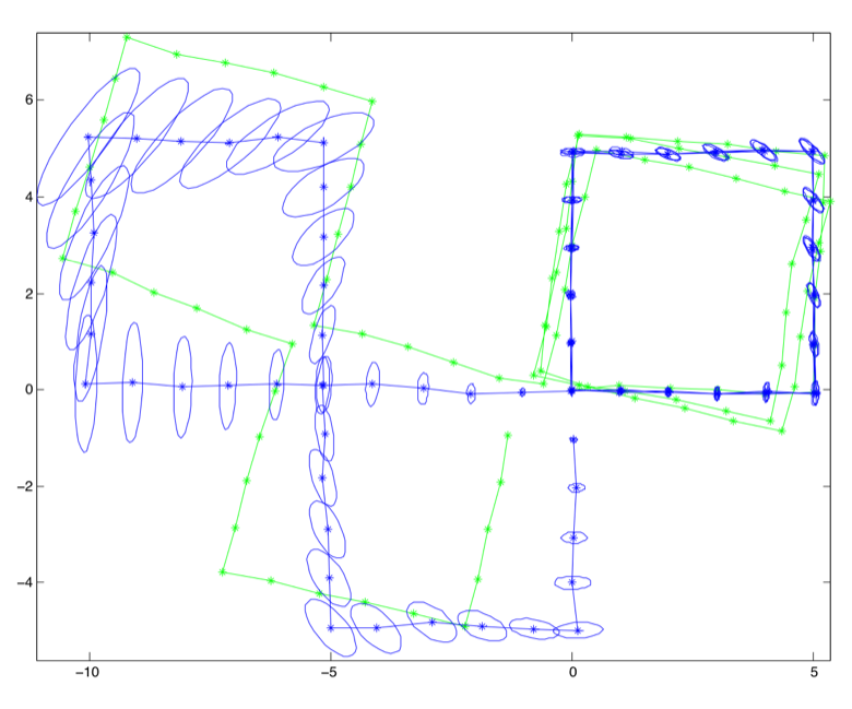
End-to-end (perception → LiDAR-in-mask → tracking → GTSAM) yields a smoother trajectory and a coherent object map. Stable IDs persist across frames; landmarks tug the pose into global consistency.

• Pose: drift reduced; turns tighten after optimization.
• Landmarks: buoys posts cluster with reasonable covariance.

System Overview

Object-centric SLAM with a GTSAM back-end.

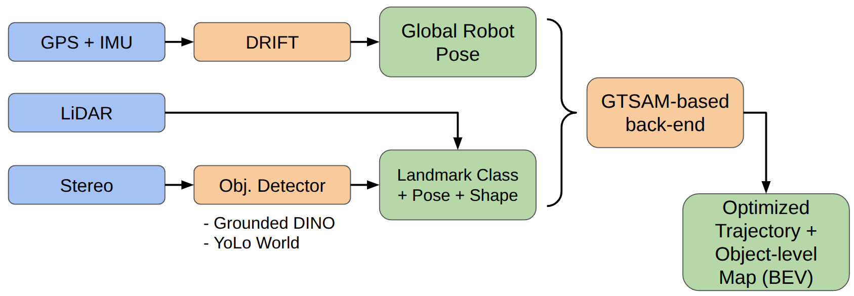
• GPS+IMU → DRIFT: supplies a global pose prior.
• LiDAR / Stereo → Detector: Grounded-SAM 2 / open-vocab models output masks, boxes, labels.
• Landmarks: class + pose/shape cues with uncertainty.
• Back-end: GTSAM optimizes poses and landmarks into a coherent object map.

Why GTSAM?

Initial estimate is shown in green. The GTSAM optimized trajectory, with covariance ellipses, is shown in blue.

GTSAM frames SLAM as a factor graph—variables linked by probabilistic factors—and solves it with Gauss-Newton/LM or iSAM2 for incremental updates. It cleanly fuses odometry and object measurements with proper noise and robust losses.

Factors in This Project

• PriorFactor<Pose2>: anchors the frame at t=0 (tight covariance).
• BetweenFactor<Pose2>: odometry as (Δx, Δy, Δθ) with Σ_odom.
• Bearing/Range factors: BearingRangeFactor<Pose2,Point2> (θ, ρ), or bearing-only when range is weak; robust loss for mask outliers.

Together: prior fixes gauge, odometry propagates motion, object factors enforce global consistency → cleaner trajectory and semantic BEV.

Perception — Open-Vocabulary Detection

YOLO-World — fast, but many false positives.

Grounded-SAM 2 — better detection and segmentation.

YOLO-World handled zero-shot prompts (buoy, dock post/face, cone, sign) but produced many false positives. Switching to Grounded-SAM 2 (GroundingDINO prompts + SAM masks) improved precision and boundary quality, so we proceed with Grounded-SAM 2. I plan to fine-tune it for maritime scenes to raise precision/recall and calibrate confidence scores.

In the future, I’ll fine-tune Grounded-SAM 2 to boost detection precision/recall and produce more calibrated confidence scores in maritime scenes.

Range from Segmentation — LiDAR Inside the Mask

For each Grounded-SAM 2 mask, LiDAR is projected into the camera, and only in-mask points are pooled. Median range and centroid form a robust per-object measurement used by tracking and SLAM.

Console print: class, 3D estimate (x, y, z in odom), and number of LiDAR points inside the mask.

For each Grounded-SAM 2 mask, LiDAR is projected into the camera, and only in-mask points are pooled. Median range and centroid form a robust per-object measurement used by tracking and SLAM.

• Projection: LiDAR → camera → pixels; keep points inside the mask polygon.
• Pooled stats: ρ = median(‖p‖), centroid ĉ = median({p_i}), quality = {N, spread (MAD/IQR)}.
• Output: {label, θ, ρ, centroid, Σ, N}; drop if N < N_min or spread too large.

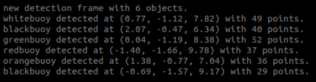
Masks give clean spatial support, so medians suppress water/glare outliers. The console summary (e.g., “greenbuoy … with 52 points”) reflects these pooled values.

Tracking Algorithm

Anisotropic uncertainty (range ≫ bearing) creates an elliptical acceptance region. Mahalanobis distance respects this; Euclidean does not.

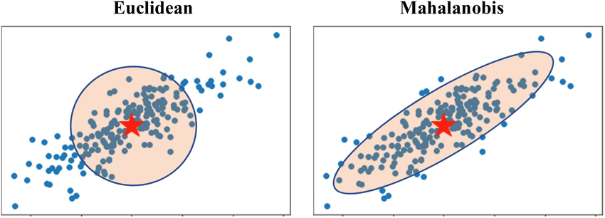
Object detections are associated to existing tracks using Mahalanobis distance. Because range is noisier than bearing in our setup (LiDAR/camera-to-odom projection), the innovation covariance is elongated along range, so we gate with an ellipse rather than a circle.

Pipeline: new measurement → predict → Mahalanobis gate → create or update → stable Track IDs.

Detections are matched to tracks with Mahalanobis gating. Because range is noisier than bearing, the innovation covariance is elongated along range, so the gate is an ellipse, not a circle.

• Predict: x_pred, P_pred
• Innovate: y = z − h(x_pred), S = H P_pred Hᵀ + R
• Gate: d² = yᵀ S⁻¹ y ≤ τ (χ² threshold)
• Assign: nearest-neighbor (or Hungarian) within gate
• Update: K = P_predHᵀS⁻¹; x = x_pred + Ky; P = (I − KH)P_pred
• Manage: create new tracks for ungated detections; age out unmatched tracks

Takeaway: Mahalanobis gating respects the uncertainty geometry, reducing false matches and stabilizing IDs for the GTSAM factors.